In [1]:
using Pkg
Pkg.activate(pwd())
Pkg.instantiate()
  Activating project at `~/Documents/github.com/ucla-biostat-216/2022fall/slides/01-intro`
In [2]:
using GraphPlot, Graphs, ImageCore, ImageIO, ImageMagick, ImageShow, 
    LinearAlgebra, MatrixDepot, MLDatasets, QuartzImageIO, 
    RDatasets, StatsModels, TextAnalysis
┌ Info: verify download of index files...
└ @ MatrixDepot /Users/huazhou/.julia/packages/MatrixDepot/T9mnt/src/MatrixDepot.jl:118
┌ Info: reading database
└ @ MatrixDepot /Users/huazhou/.julia/packages/MatrixDepot/T9mnt/src/download.jl:23
┌ Info: adding metadata...
└ @ MatrixDepot /Users/huazhou/.julia/packages/MatrixDepot/T9mnt/src/download.jl:67
┌ Info: adding svd data...
└ @ MatrixDepot /Users/huazhou/.julia/packages/MatrixDepot/T9mnt/src/download.jl:69
┌ Info: writing database
└ @ MatrixDepot /Users/huazhou/.julia/packages/MatrixDepot/T9mnt/src/download.jl:74
┌ Info: used remote sites are sparse.tamu.edu with MAT index and math.nist.gov with HTML index
└ @ MatrixDepot /Users/huazhou/.julia/packages/MatrixDepot/T9mnt/src/MatrixDepot.jl:120

Introduction

Subject of linear algebra

  • Vector $\mathbf{x} \in \mathbb{R}^{n}$: $$ \mathbf{x} = \begin{pmatrix} x_1 \\ x_2 \\ \vdots \\ x_n \end{pmatrix}. $$

  • Matrix $\mathbf{X} = (x_{ij}) \in \mathbb{R}^{m \times n}$: $$ \mathbf{X} = \begin{pmatrix} x_{11} & \cdots & x_{1n} \\ \vdots & \ddots & \vdots \\ x_{m1} & \cdots & x_{mn} \end{pmatrix}. $$

Examples of vectors and matrices

Design matrix

In statistics, tabular data is often summarized by a predictor matrix or covariate matrix or design matrix or feature matrix, which is denoted by $\mathbf{X}$ by convention. Each row of the feature matrix is an observation, and each column is a covariate/measurement/feature.

The famous Fisher's Iris data:

In [3]:
# the famous Fisher's Iris data
# <https://en.wikipedia.org/wiki/Iris_flower_data_set>
iris = dataset("datasets", "iris")
Out[3]:

150 rows × 5 columns

SepalLengthSepalWidthPetalLengthPetalWidthSpecies
Float64Float64Float64Float64Cat…
15.13.51.40.2setosa
24.93.01.40.2setosa
34.73.21.30.2setosa
44.63.11.50.2setosa
55.03.61.40.2setosa
65.43.91.70.4setosa
74.63.41.40.3setosa
85.03.41.50.2setosa
94.42.91.40.2setosa
104.93.11.50.1setosa
115.43.71.50.2setosa
124.83.41.60.2setosa
134.83.01.40.1setosa
144.33.01.10.1setosa
155.84.01.20.2setosa
165.74.41.50.4setosa
175.43.91.30.4setosa
185.13.51.40.3setosa
195.73.81.70.3setosa
205.13.81.50.3setosa
215.43.41.70.2setosa
225.13.71.50.4setosa
234.63.61.00.2setosa
245.13.31.70.5setosa
254.83.41.90.2setosa
265.03.01.60.2setosa
275.03.41.60.4setosa
285.23.51.50.2setosa
295.23.41.40.2setosa
304.73.21.60.2setosa

We can turn a tabular data set into a feature matrix according to a model formula:

In [4]:
# use full dummy coding (one-hot coding) for categorical variable Species
iris_X = ModelMatrix(ModelFrame(
    @formula(1 ~ 1 + SepalLength + SepalWidth + PetalLength + PetalWidth + Species), 
    iris,
    contrasts = Dict(:Species => StatsModels.FullDummyCoding()))).m
Out[4]:
150×8 Matrix{Float64}:
 1.0  5.1  3.5  1.4  0.2  1.0  0.0  0.0
 1.0  4.9  3.0  1.4  0.2  1.0  0.0  0.0
 1.0  4.7  3.2  1.3  0.2  1.0  0.0  0.0
 1.0  4.6  3.1  1.5  0.2  1.0  0.0  0.0
 1.0  5.0  3.6  1.4  0.2  1.0  0.0  0.0
 1.0  5.4  3.9  1.7  0.4  1.0  0.0  0.0
 1.0  4.6  3.4  1.4  0.3  1.0  0.0  0.0
 1.0  5.0  3.4  1.5  0.2  1.0  0.0  0.0
 1.0  4.4  2.9  1.4  0.2  1.0  0.0  0.0
 1.0  4.9  3.1  1.5  0.1  1.0  0.0  0.0
 1.0  5.4  3.7  1.5  0.2  1.0  0.0  0.0
 1.0  4.8  3.4  1.6  0.2  1.0  0.0  0.0
 1.0  4.8  3.0  1.4  0.1  1.0  0.0  0.0
 ⋮                        ⋮         
 1.0  6.0  3.0  4.8  1.8  0.0  0.0  1.0
 1.0  6.9  3.1  5.4  2.1  0.0  0.0  1.0
 1.0  6.7  3.1  5.6  2.4  0.0  0.0  1.0
 1.0  6.9  3.1  5.1  2.3  0.0  0.0  1.0
 1.0  5.8  2.7  5.1  1.9  0.0  0.0  1.0
 1.0  6.8  3.2  5.9  2.3  0.0  0.0  1.0
 1.0  6.7  3.3  5.7  2.5  0.0  0.0  1.0
 1.0  6.7  3.0  5.2  2.3  0.0  0.0  1.0
 1.0  6.3  2.5  5.0  1.9  0.0  0.0  1.0
 1.0  6.5  3.0  5.2  2.0  0.0  0.0  1.0
 1.0  6.2  3.4  5.4  2.3  0.0  0.0  1.0
 1.0  5.9  3.0  5.1  1.8  0.0  0.0  1.0

Grayscale images

Neural networks can classify handwritten digits in high accuracy. Each handwritten digit is represented by a grayscale image. The famous MNIST data set contains 60,000 training images and 10,000 test images. Each image is a $28 \times 28$ matrix:

In [5]:
# first training sample: image, digit label
# MNIST.traindata(1)
MNIST(split=:train)[1]
Out[5]:
(features = Float32[0.0 0.0 … 0.0 0.0; 0.0 0.0 … 0.0 0.0; … ; 0.0 0.0 … 0.0 0.0; 0.0 0.0 … 0.0 0.0], targets = 5)
In [6]:
# first training digit
X = MNIST(split=:train)[1][1]
Out[6]:
28×28 Matrix{Float32}:
 0.0  0.0  0.0  0.0  0.0  0.0        …  0.0       0.0        0.0  0.0  0.0
 0.0  0.0  0.0  0.0  0.0  0.0           0.0       0.0        0.0  0.0  0.0
 0.0  0.0  0.0  0.0  0.0  0.0           0.0       0.0        0.0  0.0  0.0
 0.0  0.0  0.0  0.0  0.0  0.0           0.0       0.0        0.0  0.0  0.0
 0.0  0.0  0.0  0.0  0.0  0.0           0.215686  0.533333   0.0  0.0  0.0
 0.0  0.0  0.0  0.0  0.0  0.0        …  0.67451   0.992157   0.0  0.0  0.0
 0.0  0.0  0.0  0.0  0.0  0.0           0.886275  0.992157   0.0  0.0  0.0
 0.0  0.0  0.0  0.0  0.0  0.0           0.992157  0.992157   0.0  0.0  0.0
 0.0  0.0  0.0  0.0  0.0  0.0           0.992157  0.831373   0.0  0.0  0.0
 0.0  0.0  0.0  0.0  0.0  0.0           0.992157  0.529412   0.0  0.0  0.0
 0.0  0.0  0.0  0.0  0.0  0.0        …  0.992157  0.517647   0.0  0.0  0.0
 0.0  0.0  0.0  0.0  0.0  0.0           0.956863  0.0627451  0.0  0.0  0.0
 0.0  0.0  0.0  0.0  0.0  0.0117647     0.521569  0.0        0.0  0.0  0.0
 ⋮                        ⋮          ⋱                       ⋮         
 0.0  0.0  0.0  0.0  0.0  0.494118      0.0       0.0        0.0  0.0  0.0
 0.0  0.0  0.0  0.0  0.0  0.533333      0.0       0.0        0.0  0.0  0.0
 0.0  0.0  0.0  0.0  0.0  0.686275      0.0       0.0        0.0  0.0  0.0
 0.0  0.0  0.0  0.0  0.0  0.101961      0.0       0.0        0.0  0.0  0.0
 0.0  0.0  0.0  0.0  0.0  0.65098    …  0.0       0.0        0.0  0.0  0.0
 0.0  0.0  0.0  0.0  0.0  1.0           0.0       0.0        0.0  0.0  0.0
 0.0  0.0  0.0  0.0  0.0  0.968627      0.0       0.0        0.0  0.0  0.0
 0.0  0.0  0.0  0.0  0.0  0.498039      0.0       0.0        0.0  0.0  0.0
 0.0  0.0  0.0  0.0  0.0  0.0           0.0       0.0        0.0  0.0  0.0
 0.0  0.0  0.0  0.0  0.0  0.0        …  0.0       0.0        0.0  0.0  0.0
 0.0  0.0  0.0  0.0  0.0  0.0           0.0       0.0        0.0  0.0  0.0
 0.0  0.0  0.0  0.0  0.0  0.0           0.0       0.0        0.0  0.0  0.0
In [7]:
# apparently it's digit 5
convert2image(MNIST, X)
Out[7]:

Color images

CIFAR-10 is a collection of 50,000 training images and 10,000 test images, each belonging to 1 of 10 mutually exclusive classes (frog, truck, ...). Each color image is represented by three channels: R (red), G (green), B (blue). Each channel is a $32 \times 32$ intensity matrix.

In [8]:
# 2nd training image in CIFAR10
X = CIFAR10(split=:train)[2].features
Out[8]:
32×32×3 Array{Float32, 3}:
[:, :, 1] =
 0.603922  0.54902   0.54902   0.533333  …  0.686275   0.647059   0.639216
 0.494118  0.568627  0.545098  0.537255     0.611765   0.611765   0.619608
 0.411765  0.490196  0.45098   0.478431     0.603922   0.623529   0.639216
 0.4       0.486275  0.576471  0.517647     0.576471   0.513726   0.568627
 0.490196  0.588235  0.541176  0.592157     0.607843   0.368627   0.168627
 0.607843  0.596078  0.517647  0.709804  …  0.631373   0.4        0.0745098
 0.67451   0.682353  0.666667  0.796078     0.627451   0.423529   0.0784314
 0.705882  0.698039  0.698039  0.815686     0.654902   0.501961   0.290196
 0.556863  0.52549   0.670588  0.815686     0.647059   0.603922   0.52549
 0.435294  0.431373  0.752941  0.796078     0.596078   0.611765   0.466667
 0.415686  0.521569  0.858824  0.701961  …  0.639216   0.713726   0.431373
 0.427451  0.639216  0.917647  0.662745     0.643137   0.701961   0.388235
 0.482353  0.752941  0.898039  0.643137     0.521569   0.490196   0.239216
 ⋮                                       ⋱             ⋮          
 0.454902  0.556863  0.694118  0.717647  …  0.243137   0.137255   0.0235294
 0.4       0.376471  0.396078  0.47451      0.2        0.0823529  0.0392157
 0.372549  0.388235  0.396078  0.356863     0.172549   0.054902   0.0980392
 0.352941  0.372549  0.345098  0.368627     0.152941   0.0431373  0.2
 0.282353  0.34902   0.403922  0.356863     0.168627   0.054902   0.266667
 0.235294  0.313726  0.368627  0.301961  …  0.4        0.231373   0.352941
 0.219608  0.254902  0.254902  0.270588     0.215686   0.192157   0.454902
 0.301961  0.329412  0.32549   0.380392     0.12549    0.211765   0.52549
 0.368627  0.360784  0.352941  0.345098     0.0901961  0.317647   0.54902
 0.356863  0.376471  0.309804  0.298039     0.164706   0.403922   0.560784
 0.341176  0.301961  0.266667  0.25098   …  0.239216   0.482353   0.560784
 0.309804  0.278431  0.262745  0.278431     0.364706   0.513726   0.560784

[:, :, 2] =
 0.694118  0.627451  0.607843  0.576471  …  0.654902  0.603922   0.580392
 0.537255  0.6       0.572549  0.556863     0.603922  0.596078   0.580392
 0.407843  0.490196  0.45098   0.47451      0.627451  0.631373   0.611765
 0.396078  0.505882  0.6       0.521569     0.6       0.509804   0.529412
 0.513726  0.631373  0.588235  0.615686     0.6       0.345098   0.12549
 0.65098   0.643137  0.568627  0.756863  …  0.603922  0.360784   0.0352941
 0.745098  0.737255  0.721569  0.870588     0.639216  0.419608   0.054902
 0.780392  0.741176  0.741176  0.890196     0.678431  0.505882   0.266667
 0.611765  0.545098  0.690196  0.87451      0.647059  0.584314   0.490196
 0.470588  0.435294  0.764706  0.858824     0.596078  0.592157   0.431373
 0.419608  0.498039  0.854902  0.760784  …  0.635294  0.694118   0.396078
 0.407843  0.611765  0.913725  0.721569     0.639216  0.686275   0.364706
 0.47451   0.752941  0.929412  0.729412     0.541176  0.505882   0.247059
 ⋮                                       ⋱            ⋮          
 0.458824  0.560784  0.694118  0.717647  …  0.25098   0.145098   0.0235294
 0.396078  0.380392  0.4       0.482353     0.207843  0.0862745  0.0352941
 0.372549  0.396078  0.403922  0.368627     0.168627  0.0470588  0.0862745
 0.34902   0.376471  0.34902   0.380392     0.141176  0.0235294  0.176471
 0.27451   0.34902   0.403922  0.368627     0.172549  0.0509804  0.25098
 0.235294  0.317647  0.372549  0.313726  …  0.423529  0.25098    0.352941
 0.223529  0.262745  0.262745  0.282353     0.219608  0.192157   0.443137
 0.305882  0.337255  0.337255  0.392157     0.101961  0.188235   0.498039
 0.376471  0.372549  0.364706  0.356863     0.054902  0.282353   0.509804
 0.372549  0.388235  0.321569  0.305882     0.133333  0.364706   0.521569
 0.352941  0.313726  0.27451   0.258824  …  0.207843  0.447059   0.52549
 0.317647  0.286275  0.270588  0.286275     0.32549   0.47451    0.521569

[:, :, 3] =
 0.733333  0.662745  0.643137  0.607843  …  0.65098   0.501961   0.470588
 0.533333  0.603922  0.584314  0.572549     0.627451  0.509804   0.478431
 0.372549  0.462745  0.439216  0.47451      0.666667  0.556863   0.521569
 0.388235  0.517647  0.623529  0.545098     0.639216  0.498039   0.490196
 0.545098  0.678431  0.635294  0.654902     0.647059  0.372549   0.12549
 0.705882  0.686275  0.603922  0.776471  …  0.670588  0.407843   0.0470588
 0.823529  0.784314  0.745098  0.878431     0.705882  0.470588   0.0745098
 0.839216  0.768627  0.752941  0.901961     0.729412  0.537255   0.27451
 0.611765  0.537255  0.686275  0.882353     0.682353  0.596078   0.478431
 0.431373  0.4       0.741176  0.85098      0.627451  0.603922   0.419608
 0.384314  0.470588  0.85098   0.776471  …  0.666667  0.701961   0.388235
 0.4       0.611765  0.933333  0.768627     0.67451   0.701961   0.356863
 0.458824  0.733333  0.921569  0.745098     0.596078  0.529412   0.243137
 ⋮                                       ⋱            ⋮          
 0.403922  0.533333  0.698039  0.752941  …  0.301961  0.172549   0.0431373
 0.32549   0.333333  0.380392  0.486275     0.270588  0.117647   0.0470588
 0.298039  0.329412  0.360784  0.341176     0.223529  0.0705882  0.0862745
 0.309804  0.341176  0.321569  0.360784     0.184314  0.0352941  0.164706
 0.270588  0.337255  0.388235  0.345098     0.223529  0.0784314  0.262745
 0.239216  0.301961  0.337255  0.258824  …  0.478431  0.301961   0.396078
 0.211765  0.235294  0.211765  0.215686     0.25098   0.227451   0.478431
 0.282353  0.298039  0.27451   0.313726     0.113725  0.203922   0.521569
 0.329412  0.313726  0.294118  0.27451      0.054902  0.286275   0.533333
 0.278431  0.305882  0.25098   0.25098      0.141176  0.376471   0.545098
 0.278431  0.243137  0.215686  0.207843  …  0.223529  0.470588   0.556863
 0.27451   0.239216  0.215686  0.231373     0.356863  0.513726   0.564706
In [10]:
# is this a truck?
convert2image(CIFAR10, X)
Out[10]:

Text data

Text data (webpage, blog, twitter) can be transformed to numeric matrices for statistical analysis as well. For example, the 29 State of the Union Addresses by U.S. presidents, from George W Bush in 1989 to Donald Trump in 2017, can be represented by a $29 \times 9610$ document term matrix, where each row stands for one speech and each column is a word that ever appears in these speeches. An entry $x_{ij}$ of the matrix counts the number of occurrences of word $j$ in speech $i$.

In [11]:
sotupath = joinpath(dirname(pathof(TextAnalysis)), "..", "test/data/sotu")
Base.Filesystem.readdir(sotupath)
Out[11]:
29-element Vector{String}:
 "Bush_1989.txt"
 "Bush_1990.txt"
 "Bush_1991.txt"
 "Bush_1992.txt"
 "Bush_2001.txt"
 "Bush_2002.txt"
 "Bush_2003.txt"
 "Bush_2004.txt"
 "Bush_2005.txt"
 "Bush_2006.txt"
 "Bush_2007.txt"
 "Bush_2008.txt"
 "Clinton_1993.txt"
 ⋮
 "Clinton_1998.txt"
 "Clinton_1999.txt"
 "Clinton_2000.txt"
 "Obama_2009.txt"
 "Obama_2010.txt"
 "Obama_2011.txt"
 "Obama_2012.txt"
 "Obama_2013.txt"
 "Obama_2014.txt"
 "Obama_2015.txt"
 "Obama_2016.txt"
 "Trump_2017.txt"
In [12]:
crps = DirectoryCorpus(sotupath)
# Donald Trump 2017 SOTU address
text(crps[29])
Out[12]:
"Thank you very much. Mr. Speaker, Mr. Vice President, Members of Congress, the First Lady of the United States, and citizens of America: Tonight, as we mark the conclusion of our celebration of Black History Month, we are reminded of our Nation's path towards civil righ" ⋯ 28704 bytes ⋯ "n me in dreaming big and bold, and daring things for our country. I am asking everyone watching tonight to seize this moment. Believe in yourselves, believe in your future, and believe, once more, in America.\n\nThank you, God bless you, and God bless the United States.\n"
In [13]:
standardize!(crps, StringDocument)
remove_case!(crps)
prepare!(crps, strip_punctuation)
update_lexicon!(crps)
update_inverse_index!(crps)
m = DocumentTermMatrix(crps)
D = dtm(m, :dense)
Out[13]:
29×9610 Matrix{Int64}:
 3  0  0  0  0  0  0  0  0  0  0  0  0  …  0  0  0  0  0  0  0  1  0   0   0
 3  0  0  0  0  0  0  0  0  0  0  0  0     0  0  0  0  0  0  0  1  0   0   0
 1  0  0  0  0  0  0  0  0  0  0  0  0     0  0  0  0  0  0  1  1  0   0   0
 0  1  0  0  0  0  0  0  0  0  0  0  0     0  0  0  0  0  0  1  0  0   0   0
 2  8  0  1  0  0  0  0  0  0  0  0  0     0  0  0  0  0  0  0  0  0   0   0
 0  0  0  0  0  0  0  0  0  0  0  0  5  …  0  1  0  0  0  0  0  0  0   0   0
 0  2  0  2  0  0  0  0  0  0  0  1  3     0  0  0  0  0  0  0  0  0   0   0
 0  2  1  0  0  0  0  0  0  0  0  0  5     0  0  0  0  0  0  0  0  0   0   0
 0  0  0  0  0  0  0  0  0  0  0  0  1     1  0  0  0  0  0  0  0  0   0   0
 0  1  0  0  0  0  0  0  0  0  0  0  2     1  0  1  0  1  0  0  0  0  67  31
 1  1  1  0  0  0  0  0  0  0  0  0  2  …  1  0  0  0  0  0  0  0  0   0   0
 1  0  1  0  0  1  0  0  0  0  0  0  0     0  0  0  0  1  0  0  0  0   0   0
 2  6  1  0  0  2  0  0  0  0  0  0  0     0  0  0  0  0  0  0  1  0   0   0
 ⋮              ⋮              ⋮        ⋱     ⋮              ⋮            
 0  3  1  3  0  2  0  0  0  0  1  0  1     0  1  0  1  0  0  0  1  0   0   0
 3  3  0  1  1  4  0  0  0  0  0  0  1     0  0  0  0  0  0  0  1  0   0   0
 1  7  0  2  1  3  0  0  0  0  0  0  0     0  0  0  0  0  0  0  1  0   0   0
 1  0  0  0  0  0  0  0  0  0  0  0  0  …  0  0  0  0  0  0  0  0  0   0   0
 3  3  1  0  2  0  0  0  0  0  0  0  0     0  0  0  0  0  0  0  0  0  45   1
 1  0  1  1  1  2  0  0  0  0  0  0  1     0  0  0  0  0  0  0  0  0  47   1
 1  0  1  0  1  0  0  0  0  0  0  0  0     0  0  0  0  0  0  0  0  0   3   0
 2  0  1  0  0  0  0  1  0  0  0  0  0     0  0  0  0  0  0  0  0  0  41   1
 2  0  1  0  0  0  2  0  0  0  0  0  0  …  0  1  0  0  0  0  0  0  0  62   7
 0  0  0  0  0  0  0  0  0  0  0  0  1     0  1  0  0  0  0  0  0  0   0   0
 0  2  0  0  1  0  0  0  0  0  0  0  0     0  0  0  0  0  0  0  0  0   0   0
 2  0  2  0  0  0  0  0  0  0  0  0  0     0  0  0  0  0  0  0  0  0   0   0
In [14]:
m.terms
Out[14]:
9610-element Vector{String}:
 "1"
 "10"
 "100"
 "1000"
 "10000"
 "100000"
 "1010"
 "102"
 "103"
 "104"
 "105"
 "108"
 "11"
 ⋮
 "zarfos"
 "zarqawi"
 "zero"
 "zeroemission"
 "zeros"
 "zimbabwe"
 "zion"
 "zone"
 "zones"
 "ј"
 "–"
 "…"

Networks

The world wide web (WWW) with $n$ webpages can be described by a connectivity matrix or adjacency matrix $\mathbf{A} \in \{0,1\}^{n \times n}$ with entry \begin{eqnarray*} a_{ij} = \begin{cases} 1 & \text{if page $i$ links to page $j$} \\ 0 & \text{otherwise} \end{cases}. \end{eqnarray*} According to Internet Live Stats, $n \approx 1.98$ billion now. The smaller SNP/web-Google data set contains a web of 916,428 pages.

In [15]:
mdinfo("SNAP/web-Google") |> show
# SNAP/web-Google

###### MatrixMarket matrix coordinate pattern general

---

  * UF Sparse Matrix Collection, Tim Davis
  * http://www.cise.ufl.edu/research/sparse/matrices/SNAP/web-Google
  * name: SNAP/web-Google
  * [Web graph from Google]
  * id: 2301
  * date: 2002
  * author: Google
  * ed: J. Leskovec
  * fields: name title A id date author ed kind notes
  * kind: directed graph

---

  * notes:
  * Networks from SNAP (Stanford Network Analysis Platform) Network Data Sets,
  * Jure Leskovec http://snap.stanford.edu/data/index.html
  * email jure at cs.stanford.edu
  * 
  * Google web graph
  * 
  * Dataset information
  * 
  * Nodes represent web pages and directed edges represent hyperlinks between them.
  * The data was released in 2002 by Google as a part of Google Programming
  * Contest.
  * 
  * Dataset statistics
  * Nodes   875713
  * Edges   5105039
  * Nodes in largest WCC    855802 (0.977)
  * Edges in largest WCC    5066842 (0.993)
  * Nodes in largest SCC    434818 (0.497)
  * Edges in largest SCC    3419124 (0.670)
  * Average clustering coefficient  0.6047
  * Number of triangles     13391903
  * Fraction of closed triangles    0.05523
  * Diameter (longest shortest path)    22
  * 90-percentile effective diameter    8.1
  * 
  * Source (citation)
  * 
  * J. Leskovec, K. Lang, A. Dasgupta, M. Mahoney. Community Structure in Large
  * Networks: Natural Cluster Sizes and the Absence of Large Well-Defined Clusters.
  * arXiv.org:0810.1355, 2008.
  * 
  * Google programming contest, 2002
  * http://www.google.com/programming-contest/
  * 
  * Files
  * File    Description
  * web-Google.txt.gz   Webgraph from the Google programming contest, 2002

---

916428 916428 5105039
In [16]:
md = mdopen("SNAP/web-Google")
md.A
Out[16]:
916428×916428 SparseArrays.SparseMatrixCSC{Bool, Int64} with 5105039 stored entries:
⣿⣿⣿⣿⣿⣿⣿⣿⣿⣿⣿⣿⣿⣿⣿⣿⣿⣿⣿⣿⣿⣿⣿⣿⣿⣿⣿⣿⣿⣿⣿⣿⣿⣿⣿⣿⣿⣿⣿⣿
⣿⣿⣿⣿⣿⣿⣿⣿⣿⣿⣿⣿⣿⣿⣿⣿⣿⣿⣿⣿⣿⣿⣿⣿⣿⣿⣿⣿⣿⣿⣿⣿⣿⣿⣿⣿⣿⣿⣿⣿
⣿⣿⣿⣿⣿⣿⣿⣿⣿⣿⣿⣿⣿⣿⣿⣿⣿⣿⣿⣿⣿⣿⣿⣿⣿⣿⣿⣿⣿⣿⣿⣿⣿⣿⣿⣿⣿⣿⣿⣿
⣿⣿⣿⣿⣿⣿⣿⣿⣿⣿⣿⣿⣿⣿⣿⣿⣿⣿⣿⣿⣿⣿⣿⣿⣿⣿⣿⣿⣿⣿⣿⣿⣿⣿⣿⣿⣿⣿⣿⣿
⣿⣿⣿⣿⣿⣿⣿⣿⣿⣿⣿⣿⣿⣿⣿⣿⣿⣿⣿⣿⣿⣿⣿⣿⣿⣿⣿⣿⣿⣿⣿⣿⣿⣿⣿⣿⣿⣿⣿⣿
⣿⣿⣿⣿⣿⣿⣿⣿⣿⣿⣿⣿⣿⣿⣿⣿⣿⣿⣿⣿⣿⣿⣿⣿⣿⣿⣿⣿⣿⣿⣿⣿⣿⣿⣿⣿⣿⣿⣿⣿
⣿⣿⣿⣿⣿⣿⣿⣿⣿⣿⣿⣿⣿⣿⣿⣿⣿⣿⣿⣿⣿⣿⣿⣿⣿⣿⣿⣿⣿⣿⣿⣿⣿⣿⣿⣿⣿⣿⣿⣿
⣿⣿⣿⣿⣿⣿⣿⣿⣿⣿⣿⣿⣿⣿⣿⣿⣿⣿⣿⣿⣿⣿⣿⣿⣿⣿⣿⣿⣿⣿⣿⣿⣿⣿⣿⣿⣿⣿⣿⣿
⣿⣿⣿⣿⣿⣿⣿⣿⣿⣿⣿⣿⣿⣿⣿⣿⣿⣿⣿⣿⣿⣿⣿⣿⣿⣿⣿⣿⣿⣿⣿⣿⣿⣿⣿⣿⣿⣿⣿⣿
⣿⣿⣿⣿⣿⣿⣿⣿⣿⣿⣿⣿⣿⣿⣿⣿⣿⣿⣿⣿⣿⣿⣿⣿⣿⣿⣿⣿⣿⣿⣿⣿⣿⣿⣿⣿⣿⣿⣿⣿
⣿⣿⣿⣿⣿⣿⣿⣿⣿⣿⣿⣿⣿⣿⣿⣿⣿⣿⣿⣿⣿⣿⣿⣿⣿⣿⣿⣿⣿⣿⣿⣿⣿⣿⣿⣿⣿⣿⣿⣿
⣿⣿⣿⣿⣿⣿⣿⣿⣿⣿⣿⣿⣿⣿⣿⣿⣿⣿⣿⣿⣿⣿⣿⣿⣿⣿⣿⣿⣿⣿⣿⣿⣿⣿⣿⣿⣿⣿⣿⣿
⣿⣿⣿⣿⣿⣿⣿⣿⣿⣿⣿⣿⣿⣿⣿⣿⣿⣿⣿⣿⣿⣿⣿⣿⣿⣿⣿⣿⣿⣿⣿⣿⣿⣿⣿⣿⣿⣿⣿⣿
⣿⣿⣿⣿⣿⣿⣿⣿⣿⣿⣿⣿⣿⣿⣿⣿⣿⣿⣿⣿⣿⣿⣿⣿⣿⣿⣿⣿⣿⣿⣿⣿⣿⣿⣿⣿⣿⣿⣿⣿
⣿⣿⣿⣿⣿⣿⣿⣿⣿⣿⣿⣿⣿⣿⣿⣿⣿⣿⣿⣿⣿⣿⣿⣿⣿⣿⣿⣿⣿⣿⣿⣿⣿⣿⣿⣿⣿⣿⣿⣿
⣿⣿⣿⣿⣿⣿⣿⣿⣿⣿⣿⣿⣿⣿⣿⣿⣿⣿⣿⣿⣿⣿⣿⣿⣿⣿⣿⣿⣿⣿⣿⣿⣿⣿⣿⣿⣿⣿⣿⣿
⣿⣿⣿⣿⣿⣿⣿⣿⣿⣿⣿⣿⣿⣿⣿⣿⣿⣿⣿⣿⣿⣿⣿⣿⣿⣿⣿⣿⣿⣿⣿⣿⣿⣿⣿⣿⣿⣿⣿⣿
⣿⣿⣿⣿⣿⣿⣿⣿⣿⣿⣿⣿⣿⣿⣿⣿⣿⣿⣿⣿⣿⣿⣿⣿⣿⣿⣿⣿⣿⣿⣿⣿⣿⣿⣿⣿⣿⣿⣿⣿
⣿⣿⣿⣿⣿⣿⣿⣿⣿⣿⣿⣿⣿⣿⣿⣿⣿⣿⣿⣿⣿⣿⣿⣿⣿⣿⣿⣿⣿⣿⣿⣿⣿⣿⣿⣿⣿⣿⣿⣿
⣿⣿⣿⣿⣿⣿⣿⣿⣿⣿⣿⣿⣿⣿⣿⣿⣿⣿⣿⣿⣿⣿⣿⣿⣿⣿⣿⣿⣿⣿⣿⣿⣿⣿⣿⣿⣿⣿⣿⣿

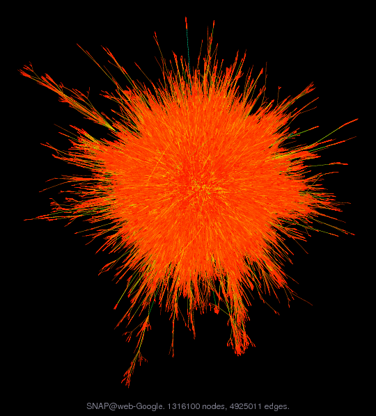
Here is a visulization of the SNAP/web-Google network
Such a directed graph can also be represented by an indicence matrix $\mathbf{B} \in \{-1,0,1\}^{m \times n}$ where $m$ is the number of verticies and $n$ is the number of edges. The entries of an incidence matrix are \begin{eqnarray*} b_{ij} = \begin{cases} -1 & \text{if edge $j$ starts at vertex $i$} \\ 1 & \text{if edge $j$ ends at vertex $i$} \\ 0 & \text{otherwise} \end{cases}. \end{eqnarray*}

Here is a directed graph with 4 nodes and 5 edges.

In [17]:
# a simple directed graph on GS p16
g = SimpleDiGraph(4)
add_edge!(g, 1, 2)
add_edge!(g, 1, 3)
add_edge!(g, 2, 3)
add_edge!(g, 2, 4)
add_edge!(g, 4, 3)
gplot(g, nodelabel=["x1", "x2", "x3", "x4"], edgelabel=["b1", "b2", "b3", "b4", "b5"])
Out[17]:
b1 b2 b3 b4 b5 x1 x2 x3 x4
In [18]:
# adjacency matrix A
convert(Matrix{Int64}, adjacency_matrix(g))
Out[18]:
4×4 Matrix{Int64}:
 0  1  1  0
 0  0  1  1
 0  0  0  0
 0  0  1  0
In [19]:
# incidence matrix B
convert(Matrix{Int64}, incidence_matrix(g))

Out[19]:
4×5 Matrix{Int64}:
 -1  -1   0   0   0
  1   0  -1  -1   0
  0   1   1   0   1
  0   0   0   1  -1

A view of statistics (or data science)

XKCD #1838