Table of Contents
Singular Value Decomposition (SVD)
using Pkg
Pkg.activate(pwd())
Pkg.instantiate()
Pkg.status()
using Images, LinearAlgebra, Random, RDatasets, StatsBase, StatsModels, StatsPlots
gr() # GR backend
We saw in earlier lectures that a square matrix can have complex eigenvalues and eigenvectors. Symmetric matrices have the nice property that all eigenvalues and eigenvectors are real. The singular value decomposition (SVD) generalizes the spectral decomposition to general rectangular matrices.
Applied mathematicians and statisticians call SVD the singularly (most) valuable decomposition.
Let $\mathbf{A} \in \mathbb{R}^{m \times n}$ with $\text{rank}(\mathbf{A})=r$. We assume $m \ge n$. Instead of the eigen-equation, now we have \begin{eqnarray*} \mathbf{A} \mathbf{v}_i &=& \sigma_i \mathbf{u}_i, \quad i = 1,\ldots,r \\ \mathbf{A} \mathbf{v}_i &=& 0 \, \mathbf{u}_i, \quad i = r+1,\ldots,n, \end{eqnarray*} where the left singular vectors $\mathbf{u}_i \in \mathbb{R}^m$ are orthonormal, the right singular vectors $\mathbf{v}_i \in \mathbb{R}^n$ are orthonormal, and the singular values $$ \sigma_1 \ge \cdots \ge \sigma_r > \sigma_{r+1} = \cdots = \sigma_{n} = 0. $$
Collecting above equations into matrix multiplication format: $$ \mathbf{A} \begin{pmatrix} \mid & & \mid & & \mid \\ \mathbf{v}_1 & \cdots & \mathbf{v}_r & \cdots & \mathbf{v}_n \\ \mid & & \mid & & \mid \end{pmatrix} = \begin{pmatrix} \mid & & \mid & & \mid \\ \mathbf{u}_1 & \cdots & \mathbf{u}_r & \cdots & \mathbf{u}_n \\ \mid & & \mid & & \mid \end{pmatrix} \begin{pmatrix} \sigma_1 & & & \\ & \ddots & & \\ & & \sigma_r & \\ & & & \mathbf{O}_{n-r} \end{pmatrix}, $$ or $$ \mathbf{A} \mathbf{V} = \mathbf{U} \boldsymbol{\Sigma}. $$ Multiplying both sides by $\mathbf{V}'$, we have the famous singular value decomposition (SVD) $$ \mathbf{A} = \mathbf{U} \boldsymbol{\Sigma} \mathbf{V}' = \sigma_1 \mathbf{u}_1 \mathbf{v}_1' + \cdots + \sigma_r \mathbf{u}_r \mathbf{v}_r', $$ where $\mathbf{U} \in \mathbb{R}^{m \times n}$ has orthogonal columns, $\boldsymbol{\Sigma} = \text{diag}(\sigma_1, \ldots, \sigma_r, \mathbf{0}_{n-r})$, and $\mathbf{V} \in \mathbb{R}^{n \times n}$ is orthogonal. $$ \mathbf{A} = \begin{pmatrix} \mid & & \mid \\ \mathbf{u}_1 & \cdots & \mathbf{u}_n \\ \mid & & \mid \end{pmatrix} \begin{pmatrix} \sigma_1 & & & \\ & \ddots & & \\ & & \sigma_r & \\ & & & \mathbf{O}_{n-r} \end{pmatrix} \begin{pmatrix} - & \mathbf{v}_1' & -\\ & \vdots & \\ - & \mathbf{v}_n' & - \end{pmatrix}. $$
# a square matrix
A = [3.0 0.0; 4.0 5.0]
# eigenvalues and eigenvectors
eigen(A)
# singular values and singular vectors
# different from eigenvalues and eigenvectors
Asvd = svd(A)
A * Asvd.Vt[1, :]
Asvd.S[1] * Asvd.U[1, :]
# orthogonality of U
Asvd.U'Asvd.U
# orthogonality of V
Asvd.V'Asvd.V
A ≈ Asvd.U * Diagonal(Asvd.S) * Asvd.V'
Reduced form of the SVD. If we just keep the first $r$ singular triplets ($\sigma_i, \mathbf{u}_i, \mathbf{v}_i$), then $$ \mathbf{A} = \mathbf{U}_r \boldsymbol{\Sigma}_r \mathbf{V}_r', $$ where $\mathbf{U}_r \in \mathbb{R}^{m \times r}$, $\boldsymbol{\Sigma}_r = \text{diag}(\sigma_1, \ldots, \sigma_r)$, and $\mathbf{V}_r \in \mathbb{R}^{n \times r}$ $$ \mathbf{A} = \begin{pmatrix} \mid & & \mid \\ \mathbf{u}_1 & \cdots & \mathbf{u}_r \\ \mid & & \mid \end{pmatrix} \begin{pmatrix} \sigma_1 & & \\ & \ddots & \\ & & \sigma_r \end{pmatrix} \begin{pmatrix} - & \mathbf{v}_1' & -\\ & \vdots & \\ - & \mathbf{v}_r' & - \end{pmatrix}. $$
Full SVD. Opposite to the reduced form of SVD, we can also augment the $\mathbf{U}$ matrix to be a square orthogonal matrix to obtain the full SVD $$ \mathbf{A} = \begin{pmatrix} \mid & & \mid \\ \mathbf{u}_1 & \cdots & \mathbf{u}_m \\ \mid & & \mid \end{pmatrix} \begin{pmatrix} \sigma_1 & & & \\ & \ddots & & \\ & & \sigma_r & \\ & & & \mathbf{O}_{n-r} \\ \\ \\ & & \mathbf{O}_{m-n, n} \end{pmatrix} \begin{pmatrix} - & \mathbf{v}_1' & - \\ & \vdots & \\ - & \mathbf{v}_n' & - \end{pmatrix}. $$
Random.seed!(216)
m, n, r = 5, 3, 2
# a rank r matrix by rank factorization
A = randn(m, r) * randn(r, n)
# svd: U is mxn, Σ is nxn, V is nxn
# SVD
svd(A)
# full SVD
svd(A, full=true)
SVD tells us everything about a matrix
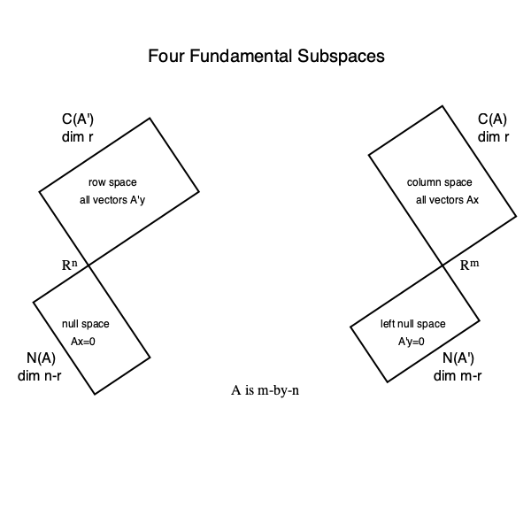
SVD and four fundamental subspaces. Given the full SVD \begin{eqnarray*} \mathbf{A} &=& \begin{pmatrix} \mid & & \mid & \mid & & \mid \\ \mathbf{u}_1 & \cdots & \mathbf{u}_r & \mathbf{u}_{r+1} & \cdots & \mathbf{u}_m \\ \mid & & \mid & \mid & & \mid \end{pmatrix} \begin{pmatrix} \sigma_1 & & & \\ & \ddots & & \\ & & \sigma_r & \\ & & & \mathbf{O}_{n-r} \\ \\ & & \mathbf{O}_{m-n, n} & \end{pmatrix} \begin{pmatrix} - & \mathbf{v}_1' & - \\ & \vdots & \\ - & \mathbf{v}_r' & - \\ - & \mathbf{v}_{r+1}' & - \\ & \vdots & \\ - & \mathbf{v}_n' & - \end{pmatrix} \\ &=& \begin{pmatrix} \mathbf{U}_r & \mathbf{U}_{m-r} \end{pmatrix} \begin{pmatrix} \boldsymbol{\Sigma}_r & & \\ & & \mathbf{O}_{n-r} \\ \\ & \mathbf{O}_{m-n,n} & \end{pmatrix} \begin{pmatrix} \mathbf{V}_r' \\ \mathbf{V}_{n-r}' \end{pmatrix}, \end{eqnarray*} Then
- $\mathcal{C}(\mathbf{A}) = \mathcal{C}(\mathbf{U}_r)$; $\quad \mathbf{U}_r \mathbf{U}_r'$ is the orthogonal projector into $\mathcal{C}(\mathbf{A})$.
- $\mathcal{N}(\mathbf{A}') = \mathcal{C}(\mathbf{U}_{m-r})$; $\quad \mathbf{U}_{m-r} \mathbf{U}_{m-r}'$ is the orthogonal projector into $\mathcal{N}(\mathbf{A}')$.
- $\mathcal{C}(\mathbf{A}') = \mathcal{C}(\mathbf{V}_{r})$; $\quad \mathbf{V}_{r} \mathbf{V}_{r}'$ is the orthogonal projector into $\mathcal{C}(\mathbf{A}')$.
- $\mathcal{N}(\mathbf{A}) = \mathcal{C}(\mathbf{V}_{n-r})$; $\quad \mathbf{V}_{n-r} \mathbf{V}_{n-r}'$ is the orthogonal projector into $\mathcal{N}(\mathbf{A})$.
$\text{rank}(\mathbf{A}) = r = \text{# positive singular values}$.
Frobenius norm $\|\mathbf{A}\|_{\text{F}}^2 = \sum_{i,j} a_{ij}^2 = \text{tr}(\mathbf{A}' \mathbf{A}) = \sum_i \sigma_i^2$.
Spectral norm or $\ell_2$ matrix norm : $\|\mathbf{A}\|_2 = \max \frac{\|\mathbf{A} \mathbf{x}\|}{\|\mathbf{x}\|} = \sigma_1$. HW7 Q3.
Random.seed!(216)
# generate a rank deficient matrix
m, n, r = 5, 3, 2
A = randn(m, r) * randn(r, n)
# full svd
Asvd = svd(A, full=true)
# Frobenius norm
norm(A) ≈ norm(Asvd.S)
# orthogonal projector to C(A)
P1 = A * pinv(A'A) * A' # WARNING: this is very inefficient code; take Biostat 257
# orthognal projector to C(A)
P2 = Asvd.U[:, 1:2] * Asvd.U[:, 1:2]'
# they should be equal by the uniqueness of orthogonal projector
P1 ≈ P2
Proof of existence of SVD using eigen-decomposition of Gram matrix
Relating SVD to eigen-decomposition. From SVD $\mathbf{A} = \mathbf{U} \boldsymbol{\Sigma} \mathbf{V}'$, we have \begin{eqnarray*} \mathbf{A}' \mathbf{A} &=& (\mathbf{V} \boldsymbol{\Sigma} \mathbf{U}') (\mathbf{U} \boldsymbol{\Sigma} \mathbf{V}') = \mathbf{V} \boldsymbol{\Sigma}^2 \mathbf{V}' \\ \mathbf{A} \mathbf{A}' &=& (\mathbf{U} \boldsymbol{\Sigma} \mathbf{V}') (\mathbf{V} \boldsymbol{\Sigma} \mathbf{U}') = \mathbf{U} \boldsymbol{\Sigma}^2 \mathbf{U}'. \end{eqnarray*} This says
- $\mathbf{u}_i$ are simply the eigenvectors of the symmetric matrix $\mathbf{A} \mathbf{A}'$
- $\mathbf{v}_i$ are simply the eigenvectors of the symmetric matrix $\mathbf{A}' \mathbf{A}$
$\sigma_i$ are simply $\sqrt{\lambda_i}$.
Proof of existence of SVD: Start from positive eigenvalues $\lambda_i > 0$ and corresponding (orthonormal) eigenvectors $\mathbf{v}_i$ of $\mathbf{A}' \mathbf{A}$. Set $\sigma_i = \sqrt \lambda_i$ and $$ \mathbf{u}_i = \frac{\mathbf{A} \mathbf{v}_i}{\sigma_i}, \quad i = 1,\ldots,r. $$ Verify that $\mathbf{u}_i$ are orthonormal. Lastly, augment $\mathbf{u}_i$s by an orthonormal basis in $\mathcal{N}(\mathbf{A}')$ and augment $\mathbf{v}_i$s by an orthonormal basis in $\mathcal{N}(\mathbf{A})$.
# revisit our earlier 5-by-3, rank-2 matrix
A
# full SVD
Asvd
eigen(A'A)
eigen(A * A')
Another relation of SVD to eigen-decomposition
In the full SVD, partition the $\mathbf{U} \in \mathbb{R}^{m \times m}$ as $$ \mathbf{U} = \begin{pmatrix} \mathbf{U}_n & \mathbf{U}_{m-n} \end{pmatrix}, $$ where $\mathbf{U}_n \in \mathbb{R}^{m \times n}$ and $\mathbf{U}_{m-n} \in \mathbb{R}^{m \times (m - n)}$. Let $\boldsymbol{\Sigma} = \text{diag}(\sigma_1, \ldots, \sigma_n)$. Then $$ \begin{pmatrix} \mathbf{O}_n & \mathbf{A}' \\ \mathbf{A} & \mathbf{O}_m \end{pmatrix} = \frac{1}{\sqrt 2} \begin{pmatrix} \mathbf{V} & \mathbf{V} & \mathbf{O} \\ \mathbf{U}_n & - \mathbf{U}_n & \sqrt{2} \mathbf{U}_{m-n} \end{pmatrix} \begin{pmatrix} \boldsymbol{\Sigma} & & \\ & - \boldsymbol{\Sigma} & \\ & & \mathbf{O}_{m-n} \end{pmatrix} \frac{1}{\sqrt 2} \begin{pmatrix} \mathbf{V}' & \mathbf{U}_n' \\ \mathbf{V}' & - \mathbf{U}_n' \\ \mathbf{O} & \sqrt{2} \mathbf{U}_{m-n}' \end{pmatrix}. $$
A
svd(A)
B = [zeros(n, n) A';
    A zeros(m, m)]
Beig = eigen(B)
# reorder eigenvalues
p = [8, 7, 6, 1, 2, 3, 5, 4]
Beigvec = Beig.vectors[:, p]
# this should be Vᵣ
Beigvec[1:n, 1:r] * sqrt(2)
# this should be Uᵣ
Beigvec[n+1:end, 1:r] * sqrt(2)
Some exercises
Question: If $\mathbf{A} = \mathbf{Q} \boldsymbol{\Lambda} \mathbf{Q}'$ is symmetric positive definite, what is its SVD?
Answer: The SVD is exactly same as eigen-decomposition $\mathbf{U} \boldsymbol{\Sigma} \mathbf{V}' = \mathbf{Q} \boldsymbol{\Lambda} \mathbf{Q}'$.
# a pd matrix
A = [1 1; 1 3]
eigen(A)
svd(A)
Question: If $\mathbf{A} = \mathbf{Q} \boldsymbol{\Lambda} \mathbf{Q}'$ is symmetric and indefinite (has negative eigenvalues), then what is its SVD?
Answer: Its SVD is $$ \mathbf{A} = \mathbf{Q} \boldsymbol{\Lambda} \mathbf{Q}' = \mathbf{Q} \begin{pmatrix} |\lambda_1| & & \\ & \ddots & \\ & & |\lambda_n| \end{pmatrix} \begin{pmatrix} \text{sgn}(\lambda_1) & & \\ & \ddots & \\ & & \text{sgn}(\lambda_n) \end{pmatrix} \mathbf{Q}'. $$
# an indefinite matrix
A = [1 2; 2 3]
eigen(A)
svd(A)
Question: Why the singular values of an orthogonal matrix $\mathbf{Q}$ are all 1?
Answer: $\mathbf{Q} = \mathbf{Q} \cdot \mathbf{I}_n \cdot \mathbf{I}_n$ is the SVD.
# Hadamard matrix of order 2
H = (1 / sqrt(2)) * [1 1; 1 -1]
# check orthogonality
H'H
# singular values are all 1
svd(H)
Why are all eigenvalues of a square matrix less than or equal to $\sigma_1$?
Answer: Recall that trthogonal matrices preserve vector length. Using the full SVD $\mathbf{A} = \mathbf{U} \boldsymbol{\Sigma} \mathbf{V}'$, $$ \|\mathbf{A} \mathbf{x}\| = \|\mathbf{U} \boldsymbol{\Sigma} \mathbf{V}' \mathbf{x}\| = \|\boldsymbol{\Sigma} \mathbf{V}' \mathbf{x}\| \le \sigma_1 \|\mathbf{V}' \mathbf{x}\| = \sigma_1 \|\mathbf{x}\|. $$ Now an eigenvector $\mathbf{x}$ satisifies $$ \|\mathbf{A} \mathbf{x}\| = |\lambda| \|\mathbf{x}\|. $$ Thus we have $|\lambda| \le \sigma_1$.
Random.seed!(216)
A = randn(5, 5)
eigvals(A) .|> abs |> sort
svdvals(A) |> sort
Question: If $\mathbf{A} = \mathbf{x} \mathbf{y}'$, find the singular values and singular vectors. What does $|\lambda| \le \sigma_1$ imply?
Answer: TODO.
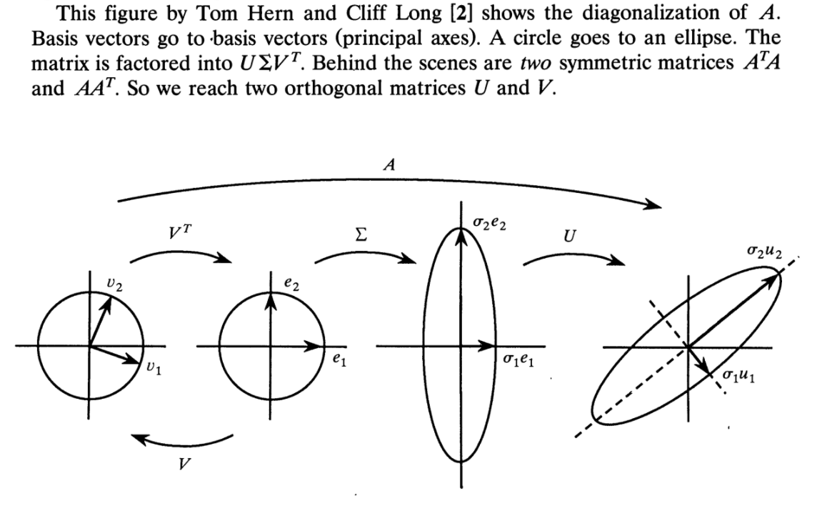
Geometry of SVD
Visualize how a $2 \times 2$ matrix acts on a vector via SVD. Picture from this paper: $$ \mathbf{A} \mathbf{x} = \mathbf{U} \boldsymbol{\Sigma} \mathbf{V}' \mathbf{x}. $$
SVD and generalized inverse
Using the SVD, the Moore-Penrose inverse) is given by
$$
\mathbf{A}^+ = \mathbf{V} \boldsymbol{\Sigma}^+ \mathbf{U}^T = \mathbf{V}_r \boldsymbol{\Sigma}_r^{-1} \mathbf{U}_r' = \sum_{i=1}^r \sigma_i^{-1} \mathbf{v}_i \mathbf{u}_i',
$$
where $\boldsymbol{\Sigma}^+ = \text{diag}(\sigma_1^{-1}, \ldots, \sigma_r^{-1}, 0, \ldots, 0)$, $r= \text{rank}(\mathbf{A})$. In HW7, you verify this definition satisifes all properties of the Moore-Pensorse inverse. This is how the pinv function is implemented in Julia, Matlab, Python, or R.
Random.seed!(216)
m, n, r = 5, 3, 2
A = randn(m, r) * randn(r, n)
Asvd = svd(A)
Asvd.Vt[1:2, :]' * Diagonal(inv.(Asvd.S[1:2])) * Asvd.U[:, 1:2]'
pinv(A)
Eckart-Young theorem: best approximation to a matrix
- Let's first look at an image compression example from https://www.mathworks.com/content/mathworks/www/en/company/newsletters/articles/professor-svd.html.
img = load("golub-561-838-rank-120.jpg")

channels = float(channelview(img))
size(channels)
channels[3, :, :]
function rank_approx(F::SVD, k)
    U, S, Vt = F.U, F.S, F.Vt
    M = U[:, 1:k] * Diagonal(S[1:k]) * Vt[1:k, :]
    M .= clamp.(M, 0.0, 1.0)
end
svdfactors = (svd(channels[1, :, :]), svd(channels[2, :, :]), svd(channels[3, :, :]))
k1, k2, k3 = 25, 25, 25
colorview(RGB,
    rank_approx(svdfactors[1], k1),
    rank_approx(svdfactors[2], k2),
    rank_approx(svdfactors[3], k3)
)

SVD has some inherent optimality properties. It prescribes how to approximate a general matrix $\mathbf{A}$ by a low rank matrix.
Before talking about approximation, we need a metric that measures the quality of approximation. We discuss 3 matrix norms.
Spectral norm or $\ell_2$ norm: $$ \|\mathbf{A}\|_2 = \max \frac{\|\mathbf{A} \mathbf{x}\|}{\|\mathbf{x}\|} = \sigma_1. $$
Frobenius norm: $$ \|\mathbf{A}\|_{\text{F}} = \sqrt{\sum_{i,j} a_{ij}^2} = \sqrt{\text{tr}(\mathbf{A}' \mathbf{A})} = \sqrt{\sigma_1^2 + \cdots + \sigma_r^2}. $$
Nuclear norm: $$ \|\mathbf{A}\|_{\text{nuc}} = \sigma_1 + \cdots + \sigma_r. $$
These 3 norms already have different values for the identity matrix: \begin{eqnarray*} \|\mathbf{I}_n\|_2 &=& 1 \\ \|\mathbf{I}_n\|_{\text{F}} &=& \sqrt{n} \\ \|\mathbf{I}_n\|_{\text{nuc}} &=& n. \end{eqnarray*} Indeed for any orthogonal matrix $\mathbf{Q} \in \mathbb{R}^{n \times n}$, \begin{eqnarray*} \|\mathbf{Q}\|_2 &=& 1 \\ \|\mathbf{Q}\|_{\text{F}} &=& \sqrt{n} \\ \|\mathbf{Q}\|_{\text{nuc}} &=& n. \end{eqnarray*}
Invariance under orthogonal transform. For all three norms, $$ \|\mathbf{Q}_1 \mathbf{A} \mathbf{Q}_2'\| = \|\mathbf{A}\| \text{ for orthogonal } \mathbf{Q}_1 \text{ and } \mathbf{Q}_2. $$
Proof: HW7.
Eckart-Young theorem. Assuming SVD of $\mathbf{A} \in \mathbb{R}^{m \times n}$ with rank $r$: $$ \mathbf{A} = \mathbf{U} \boldsymbol{\Sigma} \mathbf{V}' = \sum_{i=1}^r \sigma_i \mathbf{u}_i \mathbf{v}_i'. $$ Then the matrix $$ \mathbf{A}_k = \sum_{i=1}^k \sigma_i \mathbf{u}_i \mathbf{v}_i' $$ is the best rank-$k$ approximation to the original matrix $\mathbf{A}$ in the 3 matrix norms ($\ell_2$, Frobenius, and nuclear). More precisely, $$ \|\mathbf{A} - \mathbf{B}\| $$ is minimized by $\mathbf{A}_k$ among all matrices $\mathbf{B}$ with rank $\le k$.
Proof of Eckart-Young theorem for the $\ell_2$ norm. (optional)
First we note $$ \|\mathbf{A} - \mathbf{A}_k\|_2 = \left\|\sum_{i=1}^r \sigma_i \mathbf{u}_i \mathbf{v}_i' - \sum_{i=1}^k \sigma_i \mathbf{u}_i \mathbf{v}_i' \right\|_2 = \left\|\sum_{i=k+1}^r \sigma_i \mathbf{u}_i \mathbf{v}_i' \right\|_2 = \sigma_{k+1}. $$ We want to show that $$ \|\mathbf{A} - \mathbf{B}\|_2 = \max \frac{\|(\mathbf{A} - \mathbf{B}) \mathbf{x}\|}{\|\mathbf{x}\|} \ge \sigma_{k+1} $$ for any $\mathbf{B}$ with $\text{rank}(\mathbf{B}) \le k$. We show this by choosing a particular $\mathbf{x}$ such that $$ \frac{\|(\mathbf{A} - \mathbf{B}) \mathbf{x}\|}{\|\mathbf{x}\|} \ge \sigma_{k+1}. $$ Choose $\mathbf{x} \ne \mathbf{0}$ such that $$ \mathbf{B} \mathbf{x} = \mathbf{0} \text{ and } \mathbf{x} = \sum_{i=1}^{k+1} c_i \mathbf{v}_i. $$ There exists such $\mathbf{x}$ because (1) $\mathcal{N}(\mathbf{B})$ has dimension $\ge n-k$ because $\text{rank}(\mathbf{B}) \le k$ (rank-nullity theorem) and (2) $\mathbf{v}_1, \ldots, \mathbf{v}_{k+1}$ span a subspace of dimension $k+1$. Thus $\mathcal{N}(\mathbf{B})$ and $\text{span}\{\mathbf{v}_1, \ldots, \mathbf{v}_{k+1}\}$ has a non-trivial intersection. For this $\mathbf{x}$, we have \begin{eqnarray*} & & \|(\mathbf{A} - \mathbf{B}) \mathbf{x}\|^2 \\ &=& \|\mathbf{A} \mathbf{x}\|^2 \\ &=& \left\|\left(\sum_{i=1}^r \sigma_i \mathbf{u}_i \mathbf{v}_i'\right)\left(\sum_{i=1}^{k+1} c_i \mathbf{v}_i\right)\right\|^2 \\ &=& \left\| \sum_{i=1}^{k+1} c_i \sigma_i \mathbf{u}_i \right\|^2 \\ &=& \sum_{i=1}^{k+1} c_i^2 \sigma_i^2 \\ &\ge& \left(\sum_{i=1}^{k+1} c_i^2\right) \sigma_{k+1}^2 \\ &=& \|\mathbf{x}\|^2 \sigma_{k+1}^2. \end{eqnarray*} The proof is finished.
(Nathan Srebro's) Proof of Eckart-Young theorem for the Frobenius norm. (optional)
Let $\mathbf{B}$ be a matrix of rank $k$. By the rank factorization, $\mathbf{B} = \mathbf{C} \mathbf{R}$, where $\mathbf{C} \in \mathbb{R}^{m \times k}$ and $\mathbf{R} \in \mathbb{R}^{k \times n}$. Using SVD of $\mathbf{B}$, we will assume that $\mathbf{C}$ has orthogonal columns (so $\mathbf{C}' \mathbf{C} = \mathbf{D}$) and $\mathbf{R}$ has orthonormal rows (so $\mathbf{R} \mathbf{R}' = \mathbf{I}_k$). We want to show $\mathbf{C} = \mathbf{U}_k \boldsymbol{\Sigma}_k$ and $\mathbf{R} = \mathbf{V}_k'$, where $(\boldsymbol{\Sigma}_k, \mathbf{U}_k, \mathbf{V}_k)$ are the top $k$ singular values/vectors of $\mathbf{A}$. In order for $\mathbf{B} = \mathbf{C} \mathbf{R}$ to minimize $$ f(\mathbf{C}, \mathbf{R}) = \|\mathbf{A} - \mathbf{C} \mathbf{R}\|_{\text{F}}^2, $$ the gradient (partial derivatives) must vanish \begin{eqnarray*} \frac{\partial f(\mathbf{C}, \mathbf{R})}{\partial \mathbf{C}} &=& - 2(\mathbf{A} - \mathbf{C} \mathbf{R}) \mathbf{R}' = \mathbf{O}_{m \times k} \\ \frac{\partial f(\mathbf{C}, \mathbf{R})}{\partial \mathbf{R}} &=& - 2 \mathbf{C}' (\mathbf{A} - \mathbf{C} \mathbf{R}) = \mathbf{O}_{k \times n}. \end{eqnarray*} The first equation shows $$ \mathbf{A} \mathbf{R}' = \mathbf{C} \mathbf{R} \mathbf{R}' = \mathbf{C}. $$ Then by the second equation $$ \mathbf{A}' \mathbf{A} \mathbf{R}' = \mathbf{A}' \mathbf{C} = \mathbf{R}' \mathbf{C}' \mathbf{C} = \mathbf{R}' \mathbf{D}. $$ This says the columns of $\mathbf{R}'$ (rows of $\mathbf{R}$) must be eigenvectors of $\mathbf{A}' \mathbf{A}$, or equivalently, right singular vectors $\mathbf{v}_i$ of $\mathbf{A}$. Similarly the columns of $\mathbf{C}$ must be eigenvectors of $\mathbf{A} \mathbf{A}'$, or equivalently, left singular vectors $\mathbf{u}_i$ of $\mathbf{A}$: $$ \mathbf{A} \mathbf{A}' \mathbf{C} = \mathbf{A} \mathbf{R}' \mathbf{D} = \mathbf{C} \mathbf{D}. $$ Which $\mathbf{u}_i$ and $\mathbf{v}_i$ shall we take to minimize $f$? Apparently we should choose those with largest singular values to achieve the minimum value $\sigma_{k+1}^2 + \cdots + \sigma_r^2$.
Singular vectors and Rayleigh quotient
Goal: Maximize the Rayleigh quotient $$ \text{maximize} \quad f(\mathbf{x}) = \frac{\|\mathbf{A} \mathbf{x}\|^2}{\|\mathbf{x}\|^2} = \frac{\mathbf{x}' \mathbf{A}' \mathbf{A} \mathbf{x}}{\mathbf{x}' \mathbf{x}} = \frac{\mathbf{x}' \mathbf{S} \mathbf{x}}{\mathbf{x}' \mathbf{x}}. $$
Let's calculate the partial derivatives of the objective function $f(\mathbf{x})$ $$ \frac{\partial f(\mathbf{x})}{\partial x_i} = \frac{\left(2\sum_j s_{ij} x_j\right) (\mathbf{x}' \mathbf{x}) - (\mathbf{x}' \mathbf{S} \mathbf{x}) (2x_i)}{(\mathbf{x}' \mathbf{x})^2} = 2 (\mathbf{x}' \mathbf{x})^{-1} \left(\sum_j s_{ij} x_j - f(\mathbf{x}) x_i \right). $$ Collecting partial derivatives into the gradient vector and setting it to zero $$ \nabla f(\mathbf{x}) = 2 (\mathbf{x}' \mathbf{x})^{-1} \left[ \mathbf{S} \mathbf{x} - f(\mathbf{x}) \cdot \mathbf{x} \right] = \mathbf{0} $$ yields $$ \mathbf{S} \mathbf{x} = f(\mathbf{x}) \cdot \mathbf{x}. $$ Thus the optimal $\mathbf{x}$ must be an eigenvector of $\mathbf{S} = \mathbf{A}' \mathbf{A}$ with corresponding eigenvalue $f(\mathbf{x})$. Which one shall we choose? Apparently the top right singular vector $\mathbf{x}^\star = \mathbf{v}_1$ gives us the maximal value which is equal to $\lambda_1 = \sigma_1^2$.
In HW6, you show this result using an alternative proof (elementary linear algebra arguments).
Above we have shown $$ \max_{\mathbf{x} \ne \mathbf{0}} \frac{\|\mathbf{A} \mathbf{x}\|}{\|\mathbf{x}\|} = \sigma_1, $$ which is the spectral norm (or $\ell_2$ norm) of a matrix $\mathbf{A}$.
Random.seed!(216)
m, n, r = 5, 3, 2
A = randn(m, r) * randn(r, n)
x = randn(n)
norm(A * x) / norm(x)
Asvd = svd(A)
x = Asvd.Vt[1, :]
norm(A * x) / norm(x)
Similarly, the second right singular vector maximizes the Rayleigh quotient subject to an orthogonality constraint \begin{eqnarray*} \text{maximize} &\quad& f(\mathbf{x}) = \frac{\|\mathbf{A} \mathbf{x}\|^2}{\|\mathbf{x}\|^2} = \frac{\mathbf{x}' \mathbf{A}' \mathbf{A} \mathbf{x}}{\mathbf{x}' \mathbf{x}} = \frac{\mathbf{x}' \mathbf{S} \mathbf{x}}{\mathbf{x}' \mathbf{x}} \\ \text{subject to} &\quad& \mathbf{x} \perp \mathbf{v}_1. \end{eqnarray*}
Submatrices have smaller singular values. Let $\mathbf{B}$ be a submatrix of $\mathbf{A} \in \mathbb{R}^{m \times n}$. Then $$ \|\mathbf{B}\| \le \|\mathbf{A}\| $$ or equivalently $$ \sigma_1 (\mathbf{B}) \le \sigma_1 (\mathbf{A}). $$
Proof: Let $\tilde{\mathbf{y}} \in \mathbb{R}^n$ hold corresponding entries in $\mathbf{y}$ and be zero elsewhere. Then $$ \sigma_1 (\mathbf{B}) = \max_{\mathbf{y}} \frac{\|\mathbf{B} \mathbf{y}\|}{\|\mathbf{y}\|} \le \max_{\tilde{\mathbf{y}}} \frac{\|\mathbf{A} \tilde{\mathbf{y}}\|}{\|\tilde{\mathbf{y}}\|} \le \max_{\mathbf{x}} \frac{\|\mathbf{A} \mathbf{x}\|}{\|\mathbf{x}\|} = \sigma_1 (\mathbf{A}). $$
svd(A[1:3, 1:2])
Principal component analysis (PCA)
PCA is a dimension reduction technique that finds the most informative linear combinations of the $p$ random variables $\mathbf{X} \in \mathbb{R}^p$. Mathematically it finds the linear combinations of the $p$ random variables that have the largest variances. If we know the population covariance of the $p$ variables is $\text{Cov}(\mathbf{X}) = \boldsymbol{\Sigma} \in \mathbb{R}^{p \times p}$, then $$ \text{Var}(\mathbf{a}' \mathbf{X}) = \mathbf{a}' \text{Cov}(\mathbf{X}) \mathbf{a} = \mathbf{a}' \boldsymbol{\Sigma} \mathbf{a}. $$ Apparently the larger magnitude of $\mathbf{a}$, the large variance $\text{Var}(\mathbf{a}' \mathbf{X})$. It makes sense to maximize the normalized version $$ \text{maximize} \quad \frac{\mathbf{a}' \boldsymbol{\Sigma} \mathbf{a}}{\mathbf{a}' \mathbf{a}}. $$
Given a data matrix $\mathbf{X} \in \mathbb{R}^{n \times p}$, where there are $n$ observations of $p$ variables. We would substitute in the sample covariance matrix $$ \widehat{\boldsymbol{\Sigma}} = \frac{\tilde{\mathbf{X}}'\tilde{\mathbf{X}}}{n-1}, $$ where $\tilde{\mathbf{X}}$ is the column-centered data, and maximize the Rayleigh quotient $$ \text{maximize} \quad \frac{\mathbf{a}' \widehat{\boldsymbol{\Sigma}} \mathbf{a}}{\mathbf{a}' \mathbf{a}}. $$ From earlier discussion we know the optimal $\mathbf{a}^\star$ maximizing this Rayleigh quotient is the top eigenvector of $\widehat{\boldsymbol{\Sigma}}$, or equivalently, the top right singular vector $\mathbf{v}_1$ of $\tilde{\mathbf{X}}$, achieving the optimal value $\lambda_1$.
Similarly, right singular vectors $\mathbf{v}_k$ maximizes $$ \frac{\mathbf{a}' \widehat{\boldsymbol{\Sigma}} \mathbf{a}}{\mathbf{a}' \mathbf{a}} $$ subject to the constraint $\mathbf{a} \perp \mathbf{v}_i$ for $i =1,\ldots,k-1$.
Coumns of $$ \mathbf{V}_r = \begin{pmatrix} \mid & & \mid \\ \mathbf{v}_1 & \cdots & \mathbf{v}_r \\ \mid & & \mid \end{pmatrix} \in \mathbb{R}^{p \times r} $$ are called the principal components.
Columns of $\tilde{\mathbf{X}} \mathbf{V}_r \in \mathbb{R}^{n \times r}$ are called the principal scores.
PCA example: Fisher's Iris data
# load iris dataset
iris = dataset("datasets", "iris")
# retrieve features and labels
X_labels = convert(Vector, iris[!, 5])
# retrieve the 4 continuous features
X = (ModelMatrix(ModelFrame(
    @formula(1 ~ 1 + SepalLength + SepalWidth + PetalLength + PetalWidth + Species),
    iris,
    contrasts = Dict(:Species => StatsModels.FullDummyCoding()))).m)[:, 2:5]
# center but not scale
X̃ = zscore(X, mean(X, dims=1), ones(1, size(X, 2)))
# Xsvd.V contains the principal components
Xsvd = svd(X̃)
Xsvd.V
# compute the top 3 principal scores
Y = X̃ * Xsvd.V[:, 1:3]
# group results by testing set labels for color coding
setosa     = Y[X_labels .== "setosa"    , :]
versicolor = Y[X_labels .== "versicolor", :]
virginica  = Y[X_labels .== "virginica" , :];
# visualize first 2 principal components in 2D interacive plot
p = scatter(setosa[:, 1], setosa[:, 2], marker=:circle, linewidth=0)
scatter!(versicolor[:, 1], versicolor[:, 2], marker=:circle, linewidth=0)
scatter!(virginica[:, 1], virginica[:, 2], marker=:circle, linewidth=0)
plot!(p, xlabel="PC1", ylabel="PC2")
# visualize first 3 principal components in 3D interacive plot
p = scatter(setosa[:, 1], setosa[:, 2], setosa[:, 3], marker=:circle, linewidth=0)
scatter!(versicolor[:, 1], versicolor[:, 2], versicolor[:, 3], marker=:circle, linewidth=0)
scatter!(virginica[:, 1], virginica[:, 2], virginica[:, 3], marker=:circle, linewidth=0)
plot!(p, xlabel="PC1", ylabel="PC2", zlabel="PC3")
PCA example: genomics
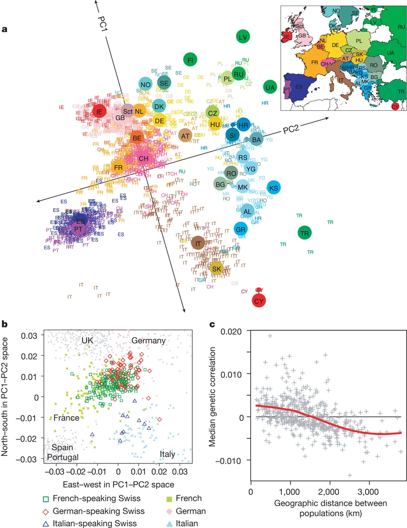
Above picture is from the article Genes mirror geography within Europe by Novembre et al (2008) published in Nature.
Matrix completion
Missing data is ubiquitous. Matrix completion (a hot topic in machine learning) aims to recover the missing values in a huge matrix.
Candes and Tao proposes a technique to complete a matrix $\mathbf{Y}$ with a large number of missing entries by an optimization problem \begin{eqnarray*} &\text{minimize}& \|\mathbf{X}\|_{\text{nuc}} \\ &\text{subject to }& x_{ij}=y_{ij} \text{ for all observed entries} y_{ij}. \end{eqnarray*} That is we seek the matrix with minimal nuclear norm that agrees with the observed entries.
See an example here.